

Risk Neutral Pricing of Options (Finance Course 3.1)
Risk Neutral Pricing of Options (Finance Course 3.1)
How to price an option using a bank account and a stock.

I originally wrote this as a Twitter thread, but I thought it might be helpful to send it out on substack as well. The style and flow might be a little different for that reason; it will be dry, but you will hopefully absorb the critical information, and I’m sure you can forgive me for the lack of literary flair you have become accustomed to.
Today the goal is to take a simple look at how options are priced. By the end, you will hopefully understand how to theoretically price an Option using the underlying stock and an interest-bearing bank account.
Let's dive into the main economic idea behind Options prices.
Pricing of random payouts has existed for a long time in the insurance industry. The way it has been priced is essentially like the formula below.

Suppose C(T) is the value of your insurance claim if your house burns down. If it wasn't random, you could discount it to get the PV, but because it needs to be random, you have to take the Expected value E subscript t, given that we have the information that we have a time t.
C(t), therefore, should be the value that the insurance company would charge you today.
The idea here is that they are in the business of selling a lot of insurance policies. To do this, they need to use the law of large numbers. They calculate that the actual value per claim will be close to its theoretical expected value.
This is not quite how it's going to work out for options. We need to find an Expected value, but it won't be under real probabilities; we must use some artificial probabilities.
So we need to change the probabilities in the model but still pretend they are accurate probabilities knowing full well they are not. Then we will calculate the expected value under those probabilities.
Why do we need to do this?
Let's look at a stock, for example.
Stock is essentially a call option with no strike price. So if the formula below (which is the same formula as above just multiplied by e-rt) is correct, it would mean that the discounted stock price today is equal to the conditional expectation of the discounted stock price in the future.
If this were correct, the discounted stock price would never change. In reality, there is no reason for that to be true. If stocks were returning the same as a risk-free instrument, why would you invest in them? You would be taking a considerable risk for a risk-free return. So, in reality, this pricing cannot hold true for all stocks.

If this were the case, we would call this a martingale process. If today's value M is equal to the expected value of the future, we can write it as below.

If we think about this in gambling terms, this is a fair gamble in which you neither lose nor win. Or, if you think about it in terms of estimation, your best estimate of what you think will happen in the future is what you see today.
Ok, so we need to look for probabilities under which discounted stock prices are martingale. See below. Probability can either be (Q or (t*)). So the expectation of the discounted future is equal to today. If we can find such a probability, they are called risk-neutral probabilities or martingale probabilities.
Roughly speaking, they are risk-neutral because it makes the stock behave on average as a risk-free instrument. (This is not quite correct but for our purposes, let's go with that for now.)

This is what we are hoping for or what we expect to have.
Note: If we wanted to look at stocks, we will simply use an S instead of a C, but we denote with C since we are talking about an insurance claim.
So how do we find some risk-neutral probability (denoted as Q.)
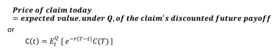
So in the formula above, we hope to have a price of a claim today C(t) (left-hand side) which is discounted by the future payoff (right-hand side).
The formula looks like it does if you have a continuously compounded risk-free rate and r is constant.
Hopefully, that makes sense, but let's answer a few questions?
How do we justify this formula? Which Q? Are there any? How many?
Here is an example using a single period binomial model.
Rate= .005
Stock (0)= 100
su = 101 (Stock goes up)
sd = 99,
We are assuming the stock went up u=1.01, and down d=.99
The goal is to price a European call with a strike price of 100.

Let’s break this down.
Again assume we are pricing a strike price of 100.

The payoff in our example is one dollar if the stock goes up and 0 dollars if the stock goes down because max{101-100} = 1, and 99-100 is negative, but you can't have a negative payout when long options so its 0.
So we are going to price this the way we have been pricing things over the past few articles by trying to replicate the payout using other methods.
In this case, we will try and replicate the payout using the stock itself and a bank account.
If we can replicate the payout of the option using the underlying and a bank account, we can use the law of one price (the cost of replicating a payout in two different ways must be the same) to price the option.
TLDR: The money you need to invest in the stock and bank account to get the same payout of the options should equal the option price itself.
Let's go,
Firstly, remember we have a payoff of 1 or 0.
The first two lines are money in the bank. Delta 0 * 1 + r. If the stock goes up 1 dollar, I will have delta 1, meaning I will have $101. If the stock goes down I'm going to have delta 1 * 99.
Goal: When it goes up, we want the payoff to be $1, and when it goes down, we want the payoff to be 0.

So here, we need to think from an option seller's perspective. The seller will need to pay 1 dollar if the stock goes up and 0 dollars if the stock goes down.
To do this, he wants to hedge in the bank and the underlying so that he has precisely 1 dollar if the stock goes up and 0 dollars if the stock goes down.
This can be solved! Its two equations and two unknowns, delta 0, and delta 1.
This is a binomial tree with only two possible values.
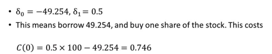
After solving, we get -49.254 in the bank and .5 in the stock (half a stock).

How would we replicate the seller of this option position? First, we need to buy .5 shares of the stock and then borrow $49.254. But borrowing that much is not enough to buy half a share; remember, a share of the stock is $100, so half a stock would cost $50.
The difference between that borrow (~$49) and the half share price ($50) is the cost of replicating this portfolio and therefore should be the price of the option.
TLDR; Using the law of one price, we should be able to replicate the payoff of the call by buying half a share of the stock using the max amount of borrowed money we are allowed to use before the payoffs diverge. The cost of this trade (difference between borrow and share price) should equal the cost of the option.
We can test this numerically by constructing an arbitrage, but we won't go into that here; we have talked about that in previous posts.
The calculations we just did are correct in theory but, in practice, are complex to implement. If this were correct, you wouldn't need options; you could construct the portfolio simply using the underlying and a bank account. But again, in practice, you would have to trade a lot, even continuously, to replicate the option. So, long story short, it's much easier to buy an option IRL.
We will continue this thought in Part II.